Example 1 (A tank reactor, batch operation)

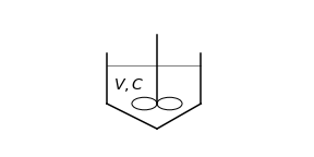
• Consider a tank containing \(V\) \(\mathrm{[m^3]}\) of water,

• which in turn contains \(C_0\) \(\mathrm{[mol \ m^{-3}]}\) of component A.

• Suppose that the concentration \(C\) \(\mathrm{[mol \ m^{-3}]}\) of A decreases at the rate

  \begin{equation} \frac{dC}{dt} = - kC \tag{1} \label{eq: example 1 problem} \end{equation}

  where \(k\) \(\mathrm{[s^{-1}]}\) is the rate constant.

• Find \(C(t)\).

Example 1, solution

• Balance, rate of

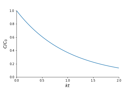
  \[{\bf \text{amount change}} = \color{gray}{\text{input} - \text{output}- {\text{production}}}- {\bf {\text{consumption}}}\]
  \[V \frac{dC(t)}{dt} = - V \left(k C\right)\]

• The equation (1) is a homogeneous constant-coefficient first order linear equation, and its solution is

  \[C(t) = C_0 \exp(-kt)\]

Example 2

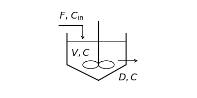
• Consider a tank containing \(V\) \(\mathrm{[m^3]}\) of water.

• We feed the tank with \(F\) \(\mathrm{[m^3 ~ s^{-1}]}\) of water with the concentration \(C_\mathrm{in}\) \(\mathrm{[mol ~ m^{-3}]}\) of component A.

• Water flow out from the tank at the same rate \(F\) (drain \(D=F\)).

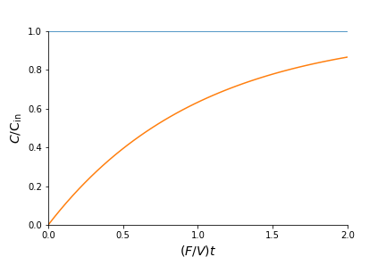
• Let the initial concentration of component A in the tank is \(0\).

• Find the change of the concentration of component A.

Example 2, solution

Example 3

• For the tank reactor in Example 2, find \(C(t)\) when the component A in tank decreases at the rate

  \[\frac{dC}{dt} = - kC\]

Example 3, solution

• This differential equation can be converted into the following form.

whose solution can be found easily,

• \(a\) and \(\kappa\) have to satisfy the following

  \[\kappa = \frac{1}{V} \left(Vk + F \right)\]
  \[\kappa a = \frac{1}{V} FC_\mathrm{in}\]

  With there equations, the differential equation is turned into

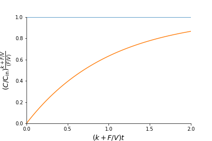
  \[\frac{d}{dt} \left( C - \frac{F/V}{k + F/V} C_\mathrm{in} \right) = - \left(k + \frac{F}{V}\right) \left(C - \frac{F/V}{k + F/V}C_\mathrm{in}\right)\]

  The initial concentration \(C_0 = 0\), thus, the solution is

  \[C(t) = \left(- \frac{F/V}{k + F/V} C_\mathrm{in}\right)\exp\left\{-\left(k+ \frac{F}{V}\right)t\right\} + \frac{F/V}{k + F/V}C_\mathrm{in}\]

Example 4

• In Example 2, what if \(C_\mathrm{in}\) is a function of \(t\), say

  \(C_\mathrm{in} = c\exp (-t)\)

  where \(c\) is a constant.

Example 4, solution

which is a first order linear (ordinary) differential equation.

• Integrating factor:

  \[\mu(t) = e^{\int^t \frac{F}{V} \, dt} = e^{tF/V}\]

• The general solution has the following form:

  \[y = \frac{1}{\mu(t)} \left\{\int \mu(t) \frac {cF}V e^{-t} \, dt + A\right\}\]

• The integral in the right hand side is evaluated as

  \begin{align*} \int \mu(t) e^t \, dt &= \int e^{tF/V}e^{-t} \, dt % \\ & = \int e^{t(F/V - 1)} \, dt \\ & = \frac1{F/V - 1} e^{t(F/V -1)} \end{align*}

• The general solution \(y\) is

  \[y = \frac{1}{e^{tF/V}}\left\{ \frac{cF}{V} \frac{1}{F/V - 1} e^{t(F/V - 1)} + A\right\}\]

• From \(C_0 = 0\), we have \(A\) as

  \[A = - \frac{c}{1 - V/F}\]

• The solution satisfying the initial condition is

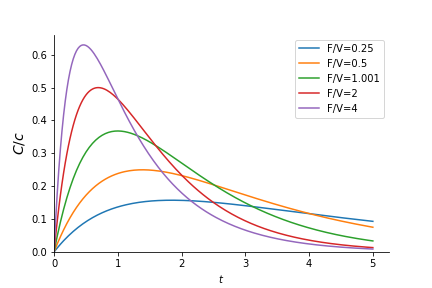
  \[C(t) = \frac{c}{V/F - 1} \left(e^{-tF/V} - e^{-t}\right)\]

Exercise 1

• In Example 4, what if

  \[C_\mathrm{in} = c(1 + \sin t)\]

  where \(c\) is a constant.